Generative Adversarial Network (GAN) Overview
Published:
Generative Adversarial Network (GAN) is a class of generative models. Basically generative models aim to model the underlying distribution of some data. Some models have the specific density function for the data distribution, while other models can only generate learned distribution via an implicit density function. GAN is one of the latter models.
Table of Content
Introduction
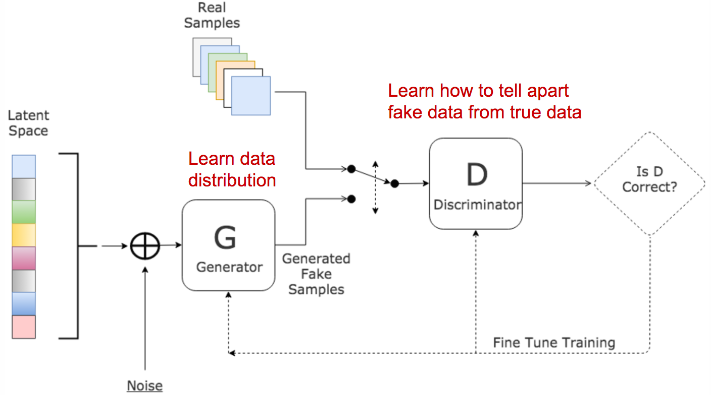
GAN is modelled as a two-player game, where one player is the generator (G) who tries to produce fake data, and another player is a discriminator (D) who tries to identify fake data from real data. The learning of the generator is from the feedback of the discriminator showing which fake data is rejected and which is accepcted by the discriminator. The learning of the discriminator is from identifying real data and fake data. The goal of the generator is to maximize the acceptance rate of its fake data. The goal of the discriminator is to maximize acceptance of real data and to minimize acceptance rate of fake data.
Model
The architecture of GAN is presented below. The input of the generator is some random noise, the output is the fake data distribution. The input of the discriminator is either real data or fake data. The discriminator learns from the errors in making decisions about real data and fake data. The generator learns from the errors in the decisions made by the discriminator about the fake data. As long as the discriminator make mistakes about decisions on fake data, the generator will learn something.
More formally, let \(p_z\) denotes the distribution over noise input \(z\), which is usually a uniform distribution or normal distribution. \(p_g\) denotes the generator distribution over \(x\) and \(p_r\) denotes the real distribution over \(x\). Here \(x, x \sim p_x(x)\) represents a real sample. \(G(z), z \sim p_z(z)\) represents a fake sample. Hence, the discriminator is to maximize its decisions over real data: \(E_{x \sim p_r(x)}[log(D(x))]\), as well as its decisions over fake data: \(E_{z \sim p_z(z)}[log(1 - D(G(z)))]\). On the other hand, the generator is to minimize identified fake data: \(E_{z \sim p_z(z)}[log(1 - D(G(z)))]\). When combinig both objectives, we are playing a minimax game with the following objective function:
\[\min_{G}\max_{D}L(D,G) = E_{x \sim p_r(x)}[log(D(x))] + E_{z \sim p_z(z)}[log(1 - D(G(z)))]\]The implementation of G and D are usually neural networks (MLP or CNN). A 50 lines code PyTorch implementation of GAN can be accessed here.
Challenges
In practice, training GAN can be quite difficult. There are primarily two challenges:
- The training may fail to converge given the loss function above
- Model collapse
The first challenge is that the model often fail to find a Nash equilibrim during training using gradient descent. One reason is that when the discriminator is optimal, the generator can not learn anything from the feedback because all its fake data are rejected. The idea that the discriminator can be optimal is that the supports of \(p_r\) and \(p_g\) lies on low dimensional manifolds and they are almost going to be disjoint, which means we can almost always separate the real and fake data perpectly.
The second challenge is that the trained generator often gets stuck into some space with low variaty and outputs the sampe data distribution.
Extensions
Unsupervised Representation Learning with Deep Convolutional Generative Adversarial Networks
This paper extends implementation of G and D into CNN. The trained DCGAN model can learn a hierachical representation of images in an unsupervised fashion. The PyTorch code can be accessed here.
Wasserstein GAN
Wasserstein GAN (WGAN) aims to alleviate the convergence problem faced by the original GAN. Specifically, the paper shows that the Jensen-Shannon divergence used in GAN is not smooth and the gradient is not continuous. Instead, the paper proposes Wasserstein distance, also known as Earth Mover’s distance, which effectively calculate the distance between two distributions by the minimum transportation needed to move from one distribution to the other distribution. The advantage of Wasserstein distance over KL or JS distances is that the gradient is continuous and smooth. The distance formula is
\[W(p_r, p_g) = \inf_{\gamma \in \prod(p_r, p_g)}E_{(x,y) \sim \gamma}[||x-y||]\]where \(\prod(p_r, p_g)\) is the set of all joint probability distributions between \(p_r\) and \(p_g\). One joint distribution \(\gamma \in \prod(p_r, p_g)\) describes one transportation plan, and the objective is to find the minimum transportation plan.
However, this objective function is intractable and the paper proposes a dual transformation to another formula, which can be optimized via gradient descent provided that the function of D is K-Lipschitz continuous:
\[|f(x_1) - f(x_2)| \leq K|x_1 - x_2|\]WGAN uses a simple weight clipping trick on D to enforce K-Lipschitz continuous. The PyTorch code can be accessed here.
References
Goodfellow, Ian, et al. “Generative adversarial nets.” Advances in neural information processing systems. 2014.
Martin Arjovsky and Léon Bottou. “Towards principled methods for training generative adversarial networks.” arXiv preprint arXiv:1701.04862 (2017).
Martin Arjovsky, Soumith Chintala, and Léon Bottou. “Wasserstein GAN.” arXiv preprint arXiv:1701.07875 (2017).
https://lilianweng.github.io/lil-log/2017/08/20/from-GAN-to-WGAN.html
https://github.com/devnag/pytorch-generative-adversarial-networks
http://www.kdnuggets.com/2017/01/generative-adversarial-networks-hot-topic-machine-learning.html