On the Convergence of Adam and Beyond

The paper On the Convergence of Adam and Beyond was awarded as the best paper on ICLR 2018. The authors empirically observed that several popular gradient based stochastic optimization algorithms such as Adam (Kingma and Ba, 2014) and RMSProp (Tieleman and Hinton, 2012), fail to converge to an optimal solution in convex settings (or a critical point in nonconvex settings). This paper identifies one cause of this convergence issue and proposes a fix to it through convergence analysis.

Specifically, this paper identifies a problem in the proof of convergence of Adam, and argues that one cause of the convergence issue is the exponential moving average used in these adaptive algorithms to scale gradient updates. In addition, this paper presents a simple one-dimensional example of Adam converging to the worst point in a convex setting, and proposes a new variant of Adam named AMSGrad that fixes the convergence issue.

Adam is one of the most widely used optimization algorithms in deep learning. Identifying and fixing the convergence issue in Adam through theoretical analysis has important practical implications. The preliminary experiments in the paper also show that AMSGrad performs slightly better than the original Adam in terms of both convergence rate and test error.

Table of Content

• Table of Content
• Problem Formulation
• Algorithms
• One-dimensional Example
• Generalizations
• Reference

Problem Formulation

The authors formulate stochastic optimization methods as online optimization problems in the full information feedback setting. Online optimization and stochastic optimization are closely related and are basically interchangeable (Cesa-Bianchi et al., 2004). For online optimization, at each time \(t \in [T]\), the algorithm picks a point (the model parameters to be learned) \(x_t \in \mathcal{F}\) , where \(\mathcal{F} \subseteq \mathcal{R}^n\) is the set of feasible points, and incurs a loss \(f_t(x_t)\), where \(f_t\) is the loss function at \(t\). In the context of machine learning, \(f_t\) is stochastic and dependent on the subsamples of data at time \(t\). The regret of the algorithm at the end of T rounds is given by

\(R_T = \sum_{t=1}^{T}f_t(x_t) - \text{min}_{x \in \mathcal{F}}\sum_{t=1}^{T}f_t(x)\),

which measures the difference between the total loss of the algorithm and the loss for an optimal fixed set of parameters. A good optimization algorithm should pick \(x_t\) such that the average regret of the algorithm approaches 0, i.e., \(\lim_{T\to\infty} R_T/T = 0\). In the paper, it is assumed that \(\mathcal{F}\) has bounded diameter and \(G_\infty = \mid \mid \nabla f_t(x)\mid \mid _{\infty}\) is bounded for all \(t \in [T]\) and \(x \in \mathcal{F}\). The aim of this paper is to essentially prove that Adam has nonzero average regret under some conditions for the hyper-parameters of Adam, and the proposed AMSGrad has zero average regret.

Gradient method is an important family of optimization methods, which are applicable to both convex and nonconvex settings. Stochastic gradient descent (SGD) is one example that is particularly popular in deep learning because it is computationally cheap and converges fast for strongly convex loss functions. The simplest gradient descent algorithm in the aforementioned online optimization formulation is to move the point \(x_t\) in the opposite direction of the gradient \(g_t = \nabla f_t(x_t)\). Specifically, the update rule is \(x_{t+1} = x_t - \alpha_t g_t\), where \(\alpha_t\) is typically set to \(\alpha/\sqrt{t}\) for some constant \(\alpha\) for theoretical convergence(Zinkevich, 2003).

Algorithms

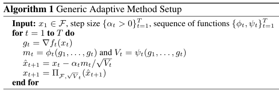
This paper focuses on adaptive gradient descent methods which can automatically adjust the magnitude of gradient update for each parameter depending on its past gradients. We can encapsulate many popular adaptive optimization algorithms in Algorithm 1 excerpted from the paper. Here \(\phi_t:\mathcal{F}^t \rightarrow \mathcal{R}^d\), \(\psi_t:\mathcal{F}^t \rightarrow \mathcal{S}_+^d\) and \(\prod\) is the projection operator, i.e., \(\prod_{\mathcal{F}, A}(y)\) for \(A \in \mathcal{S}_+^d\) is \(\text{argmin}_{x \in \mathcal{F}}\mid \mid A^{1/2}(x-y)\mid \mid\). \(\alpha_t\) is referred as step size and \(\alpha_t V_t^{-1/2}\) is the learning rate.

Algorithm 1 is the standard SGD by using \(\phi_t(g_1, ..., g_t) = g_t\) and \(\psi_t(t_1, ..., t_t) = I\).

Algorithm 1 becomes Adam by using \(\phi_t(g_1, ..., g_t) = (1-\beta_1)\sum_{i=1}^{t} \beta_1^{t-i}g_i\) and \(\psi_t(t_1, ..., t_t) = (1-\beta_2)\text{diag}(\sum_{i=1}^{t}\beta_2^{t-i}g_i^2)\) for some \(\beta_1, \beta_2 \in [0, 1)\). Alternatively, the update rule in Adam can be stated in a recursive manner: \(m_{t,i} = \beta_1 m_{t-1,i} + (1-\beta_1)g_{t,i}\), \(v_{t,i} = \beta_2 v_{t-1,i} + (1-\beta_2)g_{t,i}^2\) and \(V_t = \text{diag}(v_t)\), where \(m_0 = v_0 = \mathbf{0}\), \(i \in [d]\) and \(d\) is the number of parameters in the model.

One-dimensional Example

The authors first give an one-dimensional online convex example where \(f_t\) on \(\mathcal{F}=[-1, 1]\) is defined as

where \(C>2\). It is obvious that a convergent algorithm would eventually pick \(x_t = -1\) to minimize regret \(R_T\) because the best fixed point is \(x = -1\). Suppose \(\beta_1 = 0\), \(\beta_2 = 1/(1+C^2)\), \(\alpha_t = \alpha /t\) and \(\alpha < \sqrt{1-\beta_2}\), the optimum of Adam is proved to converge to 1 for this example, which is actually the worst point. I think this example is quite natural as it represents a typical stochastic convex loss function whose gradients are sparse. The intuition for this non-convergence is that although C provides large and informative gradients for the optimum to move towards -1, these gradients are scaled down by exponential moving average in \(\psi_t\) for the given value of \(\beta_2\).

Generalizations

To generalize the proof above, the authors prove that for any constant \(\beta_1, \beta_2 \in [0, 1)\) such that \(\beta_1 < \sqrt{\beta_2}\), there is a stochastic convex optimization problem for which Adam does not converge to the optimum. In fact, the main issue that lies in Adam is that this quantity \(\Gamma_{t+1} = \sqrt{V_{t+1}}/\alpha_{t+1} - \sqrt{V_t}/\alpha_t\) is indefinite for \(t \in [T]\), whereas the proof of convergence for Adam erroneously assume that \(\Gamma_{t+1} \succeq 0\). \(\Gamma_{t+1}\) measures the difference between the inverses of successive learning rates with respect to time. For SGD, it is easy to see that \(\Gamma_{t+1} \succeq 0\). But for Adam, it is not the case because the exponential moving average might increase the learning rate. Choosing a large \(\beta_2\) for Adam, as commonly done in practice, will help alleviate the convergence issue. In fact, by choosing variable \(\beta_2(t)\) such that \(\Gamma_{t+1} \succeq 0\) will guarantee convergence for Adam as proved in the paper.

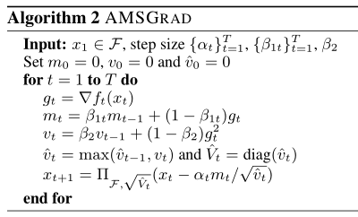
To resolve the convergence issue found in Adam with constant \(\beta_2\), the authors propose the AMSGrad in Algorithm 2. The essential difference is that AMSGrad maintains the maximum of \(v_t\) and uses this maximum value to normalize the running average of the gradients. The regret bound of AMSGrad is proved to be \(O(G_\infty \sqrt{T})\), thus the average regret bound \(\lim_{T\to\infty} R_T/T = 0\). To compare these two algorithms intuitively, suppose at a particular time step \(t\) for parameter \(i\), we have \(g_{t,i}^2 < v_{t-1,i}\), then the learning rate of Adam will increase because \(v_{t,i} = \beta_2 v_{t-1,i} + (1-\beta_2)g_{t,i}^2 < v_{t-1,i}\), however, the learning rate of AMSGrad will neither increase nor decrease because \(\tilde{v}_{t,i} = \text{max}(\tilde{v}_{t-1,i}, v_{t,i}) = \text{max}(\tilde{v}_{t-1,i}, \beta_2 v_{t-1,i} + (1-\beta_2)g_{t,i}^2) = \tilde{v}_{t-1,i}\) since \(\tilde{v}_{t-1,i} \geq v_{t-1,i} > \beta_2 v_{t-1,i} + (1-\beta_2)g_{t,i}^2\). The non-increasing property in AMSGrad avoids pitfalls of Adam. The non-decreasing property in AMSGrad avoids the slow convergence problem that the learning rate becomes extremely small over a long period of time, which actually occurs in optimization algorithms such as AdaGrad (Duchi et al., 2011).

In this post, I focus on the convergence analysis of adaptive gradient descent methods. Standard SGD methods can achieve \(\epsilon\) error within \(O(1/\epsilon^2)\) iterations. Adaptive methods perform no better than SGD in the worst case. One advantage of adaptive methods lies in better performance when gradients are sparse, in which case, learning rates for parameters with sparse gradients will be larger than parameters with dense gradients to facilitate faster convergence for sparse problems. In practice they work quite well in sparse convex problems, and even some nonconvex problems. One minor downside of the paper is that the authors do not analyze why Adam performs quite well in these problems despite its theoretical non-convergence.

Reference

Nicolo Cesa-Bianchi, Alex Conconi, and Claudio Gentile. 2004. On the generalization ability of on-line learning algorithms. IEEE Transactions on Information Theory, 50(9):2050–2057.

John Duchi, Elad Hazan, and Yoram Singer. 2011. Adaptive subgradient methods for online learning and stochas- tic optimization. Journal of Machine Learning Research, 12(Jul):2121–2159.

Diederik P Kingma and Jimmy Ba. 2014. Adam: A method for stochastic optimization. arXiv preprint arXiv:1412.6980.

Sashank J. Reddi, Satyen Kale, and Sanjiv Kumar. 2018. On the convergence of adam and beyond. In Interna- tional Conference on Learning Representations.

Tijmen Tieleman and Geoffrey Hinton. 2012. Lecture 6.5-rmsprop: Divide the gradient by a running average of its recent magnitude. COURSERA: Neural networks for machine learning, 4(2):26–31.

Martin Zinkevich. 2003. Online convex programming and generalized infinitesimal gradient ascent. In Proceed- ings of the 20th International Conference on Machine Learning (ICML-03), pages 928–936.